From Circles to Stars: Euler Diagrams with Optimized Radially Convex Boundaries
What if we could automatically visualize overlapping sets with flexible and space-efficient shapes?
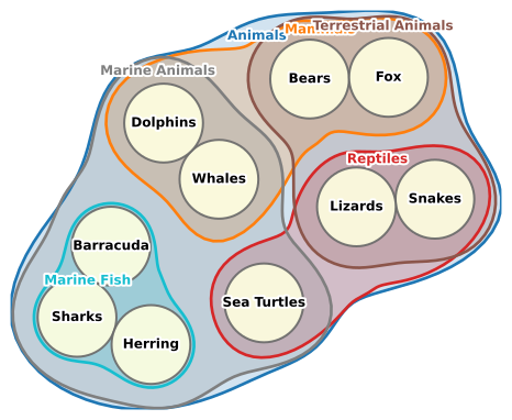
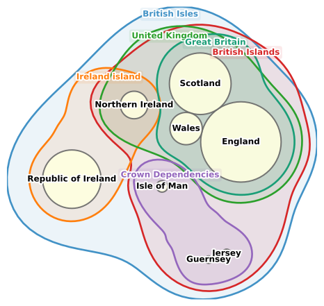
This post is about drawing Euler diagrams like the following, using mathematical optimization techniques that smoothly deform shapes to find the best possible balance between various constraints.
What are Euler diagrams?
Be it in linguistics or biology, geopolitics or mathematics, you will find sets, sets containing other sets, and sets intersecting in different ways. Things can be grouped hierarchically: Bears are mammals. Mammals are animals. But hierarchies can also overlap: Bears are also terrestrial animals, which are also animals. Whales are mammals but not terrestrial animals.
England is part of Great Britain, which is part of the United Kingdom. Northern Ireland is also part of the United Kingdom, but geographically it is part of the island called Ireland, as is the Republic of Ireland, which itself is not part of the United Kingdom. This sounds complicated, even before mentioning the Crown Dependencies. Wouldn’t it be easier to understand with a drawing?
Euler diagrams are the visual representation of these containment and intersection relations. In a sense, they are so intuitive than one cannot help but visually interpret terms like containment or intersection.
Definition:
An Euler diagram is a diagram that uses closed curves to represent sets, where spatial containment and overlap encode subset and intersection relationships.
The shape representing a subset of a given set is contained within the shape representing the superset.
Interesting fact 1: Euler diagrams are not Venn diagrams
If you thought what I just described is called a Venn diagrams, you were wrong. Venn diagrams represent every possible set intersection, including empty intersections.
This article focuses on element-level Euler diagrams: those that show individual elements within their sets, as opposed to diagrams that only represent the sets abstractly. For this type (applicable to small finite sets), the requirements are:
Shape topology: The closed shape representing each set should delimit a connected region (no disjoint pieces) without any hole. What is more, the curve delimiting this region should be simple in the sense of not intersecting itself. The shape may further be restricted to families such as polygons, circles or ellipses, and we will return to this topic.
Enclosure: Given sets A and B, if A ⊆ B, the shape for A should lie entirely inside the shape for B. Similarly, if element e belongs to set A, the shape for e should lie entirely inside the shape for A.
Intersection: the shapes for A and B should overlap if and only if A ∩ B is not empty.
Area proportionality (optional but desirable): the area of a region should be proportional to the size of the corresponding set, i.e. the number of elements it contains in the case of discrete sets.
Additional requirements can be formulated, including: two shapes should not run concurrently, or two intersecting curves should cross, not just touch etc. See Rottmann et al. (2024).
Interesting fact 2: It is impossible to draw Euler diagrams for certain set systems.
Some set systems simply cannot be drawn as Euler diagrams with connected, non-self-intersecting curves, no matter how hard you try, and this can be proven mathematically. See e.g. Rottmann et al. (2024) in the reference list for a formal treatment. Which set systems are drawable also depends on the shapes you use. Using only rectangles means you could not even draw an Euler diagram for the 3 intersecting sets in the Figure below.
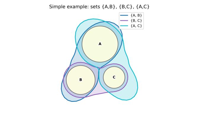
Euler diagram representing three simple sets over three elements. Try drawing the same with axis-aligned rectangles only.
Searching for the Best Primitives
While closed shape in the above definition is a wonderfully general description, which applies to circles and rectangles as well as more complex polygonal and curved regions of the plane, this generality becomes a liability when it comes to defining an algorithm that draws actual Euler diagrams.
Such an algorithms must commit to a specific family of shapes. Which family shall we choose?
Euler diagrams with circles
Euler diagrams are often composed of circles. Leibniz, Euler, Kant and Venn all drew Euler diagrams with circles. Circles are simple and nice, but also rather rigid, and they can waste a lot of space.
Consider the simplest case: two equally-sized circles of radius r, enclosed in the smallest circle that contains both. Pack them side by side and the enclosing circle has radius 2r. Its area is 4πr², while the two inner circles together cover only 2πr²: half the enclosing region is empty (more with some space between enclosed and enclosing circles), belonging to neither subset. With multiple levels of nesting this compounds: each layer inflates the container, but the added space is mostly dead area that carries no information.
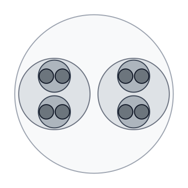
Circle-based Euler diagrams with three levels of binary nesting: the innermost (leaf) circles cover only 9% of the enclosing area. Even without offset between parent and children circles, leaf circles would cover at most 12.5% of the enclosing area.
Rectangles
Rectangles are another simple and often used candidate for set boundaries in Euler diagrams. They do pack more efficiently than circles, and can be quite useful in the context of treemaps.
Interesting fact 3: Euler diagrams are a superset of treemaps
With some imagination, you can see that treemaps are just tightly packed Euler diagrams for specific sets of sets.
If you took the animal examples and considered only phylogenetic relations, you would end up with a strictly hierarchical set of sets, which would be equivalent to a tree (with the elements as leaves). Representing parent-child relationships in trees geometrically is the idea of treemaps.
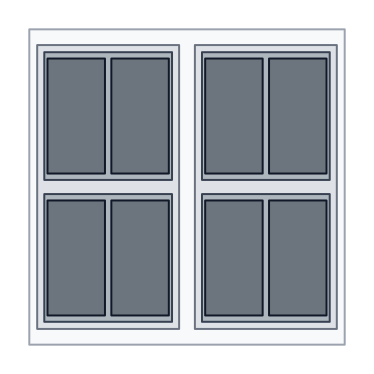 Rectangle-based Euler diagram with three levels of binary nesting, i.e. treemap: leaf rectangles now cover more than two thirds (73%) of the enclosing area, and they could cover 100% without offset between parent and children rectangles.
But rectangles do not offer much more freedom than circles and do not play too well with gradient-based optimization, which has to do with the intersection area between two rectangles being a piecewise-linear function of position, with kinks wherever an edge crosses another edge.
Crucially, the three-set example above already demonstrates the limited expressiveness of axis-aligned rectangles.
Given the limitations of circles and rectangles we just discussed, I spent a lot of time looking for a better family of shapes.
Polygons are an obvious generalization of rectangles, but they turn out to be almost too flexible: a polygon parameterized with (x_i, y_i) coordinates can intersect itself.
This is when I remembered radially convex sets.
Introducing radially convex sets
A region is radially convex if there is a center point from which every point in the region is directly visible. Imagine standing at the center of a room: if you can see every wall from that single spot, the room is star-shaped. Every convex shape qualifies, but so do many non-convex ones, including pointed stars, which is why radially convex sets are also called star-shaped.
This relates to the art gallery problem, which asks how many guards are needed to watch every point in a room. For a star-shaped room, one guard standing at the center does the job.
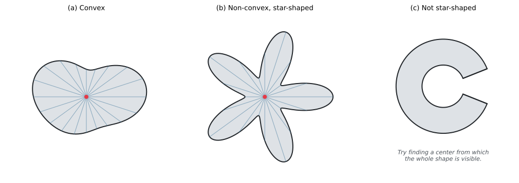 Three example shapes: convex and radially convex (left), radially convex but not convex (middle) and not radially convex (right).
Star-shaped regions admit a compact parameterization: fix a center, sample K angles uniformly in [0, 2π), and specify one radius per angle. Circles are the special case where all K radii are equal. Every other shape in the family is reachable by letting them differ.
This gives K+2 numbers per boundary, which form a fixed-size, continuous representation that can be manipulated by a gradient-based optimizer.
Smooth optimization of smooth shapes
So here is the idea: let us represent set elements with circles and sets as star-shaped radially convex sets and find the best possible arrangement of these circles and radially convex sets.
Because the boundary is a smooth function of its center and K radii, every desideratum we care about (enclosure, non-overlap, compactness etc., see below) can be written as a differentiable loss term and the whole thing handed to an optimizer.
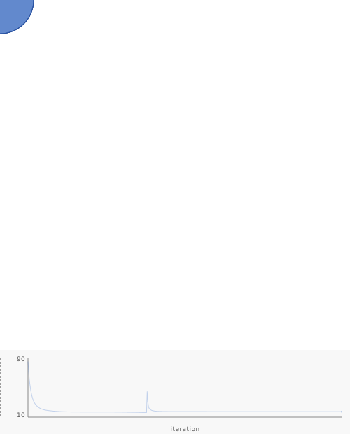 Animation of the optimization process for a 3-element/4-set example. Top: optimized shapes. Bottom: Loss curve.
Constraints and aesthetic terms
The optimizer jointly adjusts two things: the shape of each boundary (its center and K radii) and the positions of the element circles. The total loss is a weighted sum of terms which can be grouped in three categories: hard constraints, aesthetic objectives and regularization.
Hard constraints.
These constraints are non-negotiable and carry high weights. Violations are penalized both linearly (already significant penalties for small violations) and quadratically (harsh penalties for large violations).
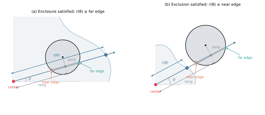
Enclosure checks that every member circle is inside its boundary: for each ray angle, it computes the minimum radius that would just graze the circle at that angle, and penalizes any shortfall.
Exclusion is the mirror image: for each non-member circle, it penalizes any radius that reaches into it.
Circle collision prevents circles from overlapping each other as they move.
See How do the enclosure and exclusion checks work? in the appendix for more information.
Aesthetic objectives.
These terms push toward compact shapes.
Area penalizes fat blobs or otherwise large shapes.
Perimeter penalizes elongated or wiggly outlines.
Smoothness penalizes squared differences between adjacent radii, discouraging jagged outlines.
The following figure illustrates the impact of different objective terms and their interplay: A high area weight causes the optimized shape to shrink. A high perimeter weight tends to straighten curve segments. A high smoothness weight lets the boundary round off.
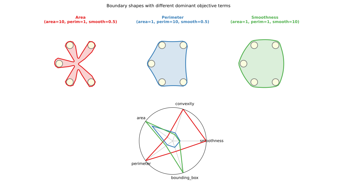
Optimization results obtained by turning up the weights of area (left), perimeter (middle), smoothness (right), while keeping circles at fixed positions.
Regularization.
Min-radius keeps boundaries from collapsing to a point or (worse) radii from becoming negative.
A convexity term can be used to penalize concavities (dents in the shape).
Position anchor can prevent circles from drifting far from their initial positions, which may (e.g. in the case of geographic entities) or may not carry meaning.
Implementation
I have implemented all this in Python using JAX, allowing for automatic differentiation and Just-in-time (JIT) compilation. Automatic differentiation means you can focus on defining and parameterizing the objective terms without having to worry about gradients. JIT compilation means you can run a gradient-based optimizer (e.g. Adam) for a few thousand iterations in seconds rather than minutes.
This is available in my vizopt package (mathematical optimization for data visualization, still in early stage), so you can also try it at home, starting from the code example in the appendix.
Conclusions
I have often advocated for the use of mathematical optimization in data visualization. In the case of the Euler diagrams presented here, without a natural algorithm to deterministically construct an Euler diagram for an arbitrary set system (do you know one?), optimization is the only real path, much more than a way to improve on a baseline. And I find that the results are visually convincing. After months of looking at Max Fürbringer’s wonderful tree of bird species in cross section and wondering how the preparation of such beautiful diagrams could be automated, it has been a delight coming closer to that goal.
So while this mathematical optimization of radially convex sets does require some effort, both in terms of configuration (lots of weights to tune) and in terms of computation (up to half a minute of optimization for larger set systems), it is worth it for me.
Nevertheless, do not assume that an Euler diagram is always the best way to visualize overlapping sets.
Interesting fact 4: Even where Euler diagrams are possible, there may be a better way to represent overlapping sets
Matrix-based representations, node-link diagrams or overlays on other visualizations can also be used and are often preferable, especially if the number of sets and elements becomes large.
References and related work
Interesting fact 5: Overlapping sets are the same as hypergraphs
Hypergraphs generalize the concept of a graph, by allowing an edge (hyperedge) to connect any number of nodes instead of two nodes for a normal graph. A hyperedge connects nodes just as a set can contain elements. The hypergraph notation can allow useful mathematical tools to be applied, as in Rottmann et al.
Alsallakh, B., Micallef, L., Aigner, W., Hauser, H., Miksch, S., & Rodgers, P. (2016). The state‐of‐the‐art of set visualization. In Computer Graphics Forum (Vol. 35, No. 1, pp. 234-260).
The Euler diagram Wikipedia article is a good read and contains an oval-based Euler diagram of terminology of the British Isles which I reproduced (in better, I would argue) with radially convex sets at the start of the article.
My
vizoptpackage: GitHub repository and documentation.
Appendix
Code example
import numpy as np

from vizopt.base import OptimConfig
from vizopt.templates.euler.stars_vs_circles import EulerDiagram

# Three elements as circles: [cx, cy, radius]
circles = np.array(
    [
        [0.0, 0.5, 0.2],  # a
        [0.5, 0.5, 0.2],  # b
        [1.0, 0.5, 0.2],  # c
    ]
)

# Four sets
sets = [[0, 1], [1, 2], [0, 2], [0, 1, 2]]  # {a,b}, {b,c}, {a,c}, {a, b, b}

diagram = EulerDiagram(
    circles,
    sets,
    set_names=["S1", "S2", "S3", "S4"],
    weight_position_anchor=0.0,
    offsets=[[0.05], [0.1], [0.15], [0.2]],
)
diagram.optimize(optim_config=OptimConfig(n_iters=5000, learning_rate=0.003))
diagram.plot()
How do the enclosure and exclusion checks work?
In plain terms:
- enclosure means the boundary of the set must reach past the far side of the circle along each ray.
- exclusion means it must stop before the near side.
More precisely: for each angle θ, project the vector from the set center to the circle center onto the ray: the along-ray component is tang and the perpendicular offset is perp. The circle’s shadow along that ray spans from tang − √(r² − perp²) (near edge) to tang + √(r² − perp²) (far edge). Enclosure requires the boundary radius to reach the far edge; exclusion requires it to stop before the near edge.
This works efficiently because the moving elements are circles. A star-vs-star intersection has no closed form: it would require comparing two full polygons, an operation roughly K times heavier per pair. Keeping the circles as circles and only the boundaries as stars is thus justified by runtime efficiency. Besides, it visually differentiates elements from sets.
Advanced topic 1: Representation
The main text describes the simplest boundary representation: K radii at uniformly-spaced angles, one optimisation variable per angle. This discrete representation has maximum freedom, allowing any star-shaped polygon to be reached. Still, we are often not interested in any star-shaped polygon but rather tend to prefer smooth polygons. While this can be enforced using the smoothness penalty term, alternative representations with built-in smoothness are also available:
A Fourier representation encodes the boundary as r(θ) = a₀ + Σ aₖcos(kθ) + bₖsin(kθ): with M harmonics, you get a C∞-smooth curve in only 2M+1 parameters, and make high-frequency wrinkles structurally impossible.
A B-spline representation uses a uniform periodic cubic spline with N control points, giving C²-smooth boundaries and local control: unlike with the Fourier representation, moving one control point only reshapes a nearby arc, not the whole boundary.
Advanced topic 2: Curriculum learning
Gradient descent is good at going downhill but bad at escaping local minima. For Euler diagrams, local minima often correspond to tangled layouts where circles belonging to the same set are separated by circles from sets to which they do not belong.
A technique called curriculum learning, by analogy with the pedagogical idea of presenting easy material before hard material, can avoid or alleviate local minima by introducing terms gradually over the course of the optimization run. Hard constraint terms (exclusion, enclosure, circle collision) can start small to allow circles to escape bad configuration before ramping up. Meanwhile, one can use a set-attraction term pulling circles towards the sets they belong to as a relaxation term that initially helps the optimization to find a rough grouping, and is subsequently ramped down.